Some time ago I was frustrated by analyzing my first selfmade data set on the university, because of the dance of the p-values. But not only p-values were frustrating me but also the task from superiors to test a Nullhypothesis, which I hade to realize was not possible by using the mainstream statistic.
But now I’ve made my own way to solve this problem by using something very insane and sinister: Bayesian Statistic…
Packages
In the following chunk you’ll find the packages I’ve used. The rio package is used to get the data from my own github account.
## To install rio use:
# library(devtools)
# install_github("leeper/rio")

library(rio)
library(ggplot2)
library(arm)
library(reshape)
library(BayesFactor)
Importing and Preparing Data
The data I will use here is about something also very sinister, it is about the Corsi Test. We wanted to test if there is no difference by doing three different versions of the Corsi Test (TS A, TS B, TS C). The participants of the study had to do all three conditions of the Corsi-Test.
Corsi.data <-import("https://raw.githubusercontent.com/MattiMeyer/Empra2/master/Daten%2Beingelesen-1.csv")

Corsi.data <- Corsi.data[c(1,9,11,13)] ## extracting the important variables
names(Corsi.data)[1] <- "ID"           ## changing one german label to english

head(Corsi.data)
##   ID TS A TS B TS C
## 1  1   36   36   25
## 2  2   63   36   42
## 3  3   56   56   80
## 4  4   30   16   25
## 5  5   88   70   63
## 6  6   72   63   88
Plotting the data
First we want to get a descriptive look at the data we’ve got and mabye to see a trend in the data:
ggplot(aes(x=values, y=..density..,fill=ind),data = stack(Corsi.data[-1]))+
 geom_density()+
 facet_grid(ind~.)+
 labs(title="Density plot of Corsi data")+
 scale_fill_discrete(name = "Group", labels = c("TS A", "TS B", "TS C"))
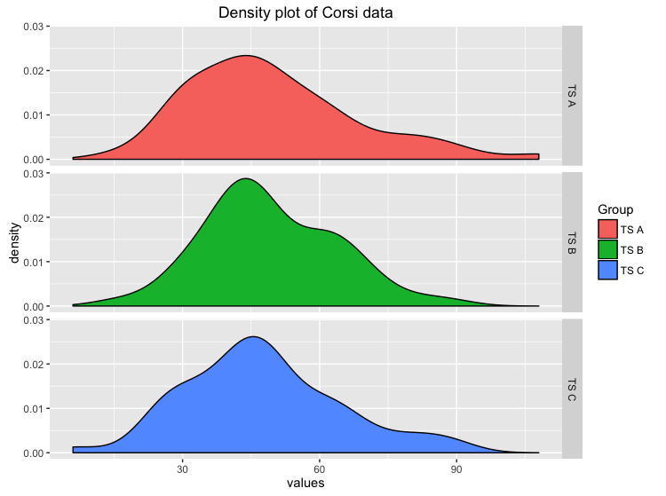
Just by looking at the distributions we could say that there is not such a big difference, but our eyes can be deceived. Well we need more to prove our Hypothesis of no difference!
Plotting the Posterior Distributions
To get a better view on the data will use the sim function of the arm package (Gelman & Hill, 2006), which simulates us a posterior distribution (Korner-Nievergelt et. al, 2015). The sim function samples pairs of random values of the parameters of the model by using an uninformative prior.
First we have to specify our linear model:
y  <- stack(Corsi.data[-1])$values
group <- stack(Corsi.data[-1])$ind

mod <- lm(y~group)
mod
##
## Call:
## lm(formula = y ~ group)
##
## Coefficients:
## (Intercept)    groupTS B    groupTS C
##     49.7115      -0.4808      -2.3077
Using the sim package
Now we will simulate the posterior distributions of our parameters of the model we build above, using 50000 iterations:
nsim <- 50000 ## number of iterations
bsim <- sim(mod,n.sim=nsim)

## values of the distributions
m.gA <- coef(bsim)[,1]
m.gB <- coef(bsim)[,1] + coef(bsim)[,2]
m.gC <- coef(bsim)[,1] + coef(bsim)[,3]
Credible interval
It would be nice to see if these distributions really show now difference. So we will calculate the credible intervals (if you don’t know the difference of confidence and credible intervals look here):
quantile(m.gA,prob=c(0.025,0.975))
##     2.5%    97.5%
## 45.08839 54.34758
quantile(m.gB,prob=c(0.025,0.975))
##     2.5%    97.5%
## 44.58671 53.84648
quantile(m.gC,prob=c(0.025,0.975))
##     2.5%    97.5%
## 42.78209 52.02371
As you can see, also the credible intervals are nearly the same! I would like to visualize this too:
## long format for graphics
posterior_long  <- stack(data.frame(m.gA,m.gB,m.gC)) ## long format of the posterior distributions
posterior_long[,2] <- c(rep(c("A"), 50000),rep(c("B"), 50000),rep(c("C"), 50000)) ## Number of groups for the three different groups of Corsi test

dim(posterior_long)
## [1] 150000 2
names(posterior_long)
## [1] "values" "ind"
## getting the credible intervals as vectors for graphics
q.m.gA <- as.vector(quantile(m.gA,prob=c(0.025,0.975)))
q.m.gB <- as.vector(quantile(m.gB,prob=c(0.025,0.975)))
q.m.gC <- as.vector(quantile(m.gC,prob=c(0.025,0.975)))

## data to plot the CrI in different grids in ggplot2
vline.dat.lower <- data.frame(ind=levels(factor(posterior_long$ind)), vl=c(q.m.gA[1],q.m.gB[1],q.m.gC[1])) ## lower CrI intervals in data frame
vline.dat.upper <- data.frame(ind=levels(factor(posterior_long$ind)), vl=c(q.m.gA[2],q.m.gB[2],q.m.gC[2])) ## upper CrI intervals in data frame

## the plot
ggplot(aes(x=values, y=..density..,fill=ind),data = posterior_long)+
 geom_density()+
 facet_grid(ind ~.)+
 geom_vline(aes(xintercept= vl),data = vline.dat.lower,colour="black",linetype=2,size=1)+
 geom_vline(aes(xintercept= vl),data = vline.dat.upper,colour="black",linetype=2,size=1)+
 labs(title= "Density plot of posterior distributions of Corsi data")+
 scale_fill_discrete(name = "Group", labels = c("TS A", "TS B", "TS C"))

Bayes Factor
Everything you saw before supports my hypothesis that there is really no difference in the three variations of the Corsi-Test, but that were just descriptive things and hard to interprete. For my own misery I’m just focused on something like the p-values in the frequentist statistic, something that shows everything that is important in one little number.
What I’ve found is the Bayes Factor (Schönbrodt et. al, 2015), which allows to analyze if the data fits more to the H0 or to the H1. The Bayes Factor is also easy to interprete because values larger as 1 support the H1 and lower 1 support the H0. For an overview of the interpretation look here. To compute the Bayes Factor you can use the BayesFactor package.
## getting data into long format
Corsi_long <- melt(Corsi.data, id=c("ID"))

## for the anovaBF function we need the ID as a factor
Corsi_long$ID <- factor(Corsi_long$ID)

bf <-  anovaBF(value ~ variable + ID, data = Corsi_long, whichRandom="ID")
bf
## Bayes factor analysis
## --------------
## [1] variable + ID : 0.09652802 ±0.73%
##
## Against denominator:
##   value ~ ID
## ---
## Bayes factor type: BFlinearModel, JZS
So the BF is 0.097 but the proportional error (~1%) is very high and I would like to reduce it by using more Monte Carlo Samples (on default 10000 are used):
newbf <-  recompute(bf, iterations = 500000)

newbf
## Bayes factor analysis
## --------------
## [1] variable + ID : 0.09721717 ±0.26%
##
## Against denominator:
##   value ~ ID
## ---
## Bayes factor type: BFlinearModel, JZS
As you can see the BF is 0.097 with a proportional error of ~0.26%, which can be interpreted as an strong evidence for the H0. So this was a Nullhypothesistest as it’s best. There is now difference in the variations of the Corsi Test. So who wants to know this? Maybe nobody, but I can sleep again…